Data Structures: Now a days A computer is involved in our day to day lives. The computer has limited memory. We must utilize limited memory in proper ways for such reason we use data structures.
Data structure consists of a base storage method and one or more algorithms that are used to access or modify the data.
A Data is an important information about an entity.
A Record is a collection of data.
A File is a collection of Records.
A Logical or Mathematical description of data in the database is known as Data Structure.
A data structure is used for quantitative analysis of the structure, which includes determining the amount of memory needed to store the structure and the time required to process the structure.
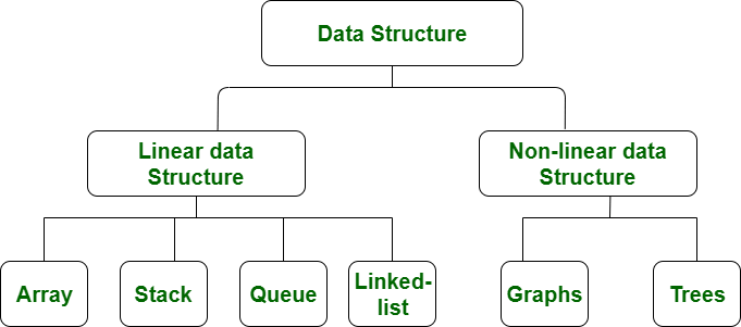
Data structure focuses on the Organization of data. It can be organized in many ways that means various data structures are used for organizing the data in the database. We categorize our data structures into two categories:
1. Linear Data Structures
2. Non-Linear Data Structures
1. Linear Data Structures: Those data structures in which data elements are organized in some sequence are called as linear data structures. For example Array, Stack, Queue & Linked List etc.
2. Non-Linear Data Structures: Those data structures in which data elements are organized in an arbitrary order or they are not organized in any sequence are called as Non-Linear Data Structures. For example Tree & Graph.

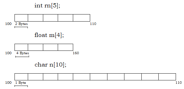
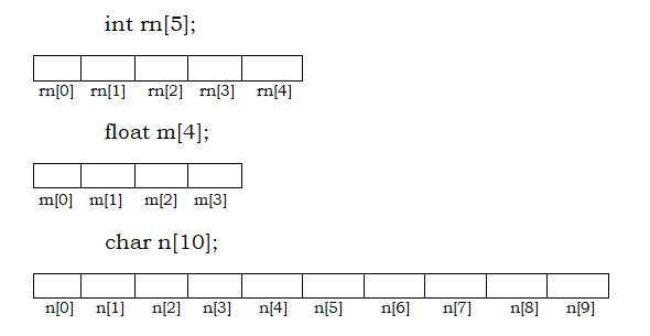
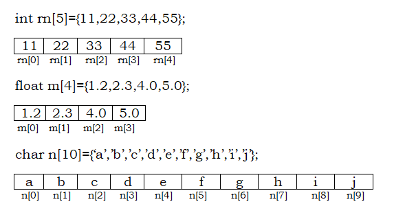
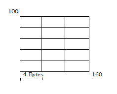
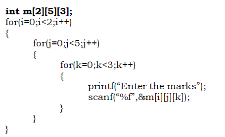
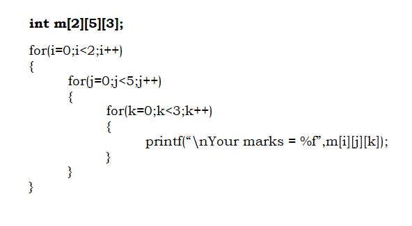
1. Array: A collection of homogenous data elements is known as Array. All the elements of an array share common name and stored on contiguous locations. Array is a Linear Data Structure.
2. Stack: It is a Linear Data Structure. A stack is also called as LIFO (Last In First Out) List. A list in which insertions and deletions can take place only on same place (One End), is known as Stack. That same place is known as Top of the Stack.
3. Queue: It is a Linear Data Structure. A queue is also called as FIFO (First In First Out) List. A list in which insertions can take place only at one end, called as Rear of the List and deletions can take place only on another end, called as Front of the List, is known as Queue.
4. Linked List: It is also a Linear Data Structure. It is a special type of List in which every element is represented as a node of list. In other words we can say that a Linked list is a collection of nodes. Every node is divided into two parts: INFO part and LINK field. INFO part of the node contains the information about the node and LINK field, also known as NEXTPOINTER field, contains the address of next node.
5. Graph: It is a non-linear data structure. A Graph is a special type of data structure that contains two things: Edges & Vertices. Any edge may go from one vertex to another vertex anywhere without any condition. We can define it another ways, branches in graph may be scattered as well as met together.
6. Tree: It is a non-linear data structure. A Tree is a special type of data structure that contains nodes. We can define it another ways, A Tree is special kind of graph which follows the rules defined below: Branches in the Tree are always scattered but not met together.
Various Common Operations on Data Structures:
All the data structures follow the common operations that are as follows:
1. Creating: The first and basic operation of data structure is Creating any structure. This operation is used to reserve the memory for elements of data structure.
2. Traversal: The elements of data structure are to be accessed as required, for same purpose we use the term Traversal. To go through each and every item in any data structure is known as Traversal Operation.
3. Insertion: The Addition of elements in data structures are to be made as required, for same purpose we use the term Insertion. To add one or more items on desired location in the data structure is known as Insertion Operation.
4. Deletion: The removal of elements in data structures are to be made as required, for same purpose we use the term Deletion. To remove one or more items on desired location in the data structure is known as deletion Operation.
5. Updating: This is an operation of changing the existing value of elements in data structures as required, for same purpose we use the term Updating. To change one or more items in the data structure is known as Update Operation.
6. Searching: The Locations of elements of data structures are to be found as required, for same purpose we use the term Searching. To find the location of desired item in the data structure is known as Search Operation.
7. Sorting: The arrangements of the elements in data structures are to be made as required, for same purpose we use the term Sorting. To rearrange the elements of any data structure in desired order is known as Sort Operation. Desired order may be Ascending or Descending.
8. Merging: The operation used when elements of two different sorted lists, composed of similar elements, are combined to form a new sorted list is called merging operation on the data structures.

Array: Array is a Linear Data Structure. A collection of homogenous data elements is known as Array. All the elements of an array share common name and stored on contiguous locations.
Arrays are categorized into 3 categories:
1. Single Dimensional Array.
2. Two Dimensional Array.
3. Multi Dimensional Array.
Single Dimensional Array (SDA): it is also known as One Dimensional Array (1D). All the elements of this type of Array are stored in one dimension only. For example: A collection of Roll Nos of 5 students(int), A collection of marks in 4 subjects(float) etc.
Declaration of SDA:
Syntax: datatype arrayname[size];
For example: To declare Roll Nos. of 5 Students(in integer form):
int rn[5];
To declare Marks of 4 Subjects(in float form):
float m[4];
To declare Name of 10 characters(in character form):
char n[10];
Memory Allocation:

Indexing or Subscripting:
Indexing always starts from 0 and goes up to n-1. Where n is the size of array.

Initialization:

Inputting:
int rn[5];
for(i=0;i<5;i++)
{
printf(“Enter the rn ”);
scanf(“%d”,&rn[i]);
}
Outputting:
int rn[5];
for(i=0;i<5;i++)
{
printf(“\nYour rno is %d”,rn[i]);
}
Two Dimensional Array (2DA): it is also known as Double Dimensional Array (DDA). All the elements of this type of Array are stored in two dimensions(i.e. rows & columns) only. For example: A collection of marks of 5 students in 3-3 subjects (float) etc.
Declaration of DDA:
Syntax: datatype arrayname[row][col];
For example: To declare Marks of 5 Students in 3-3 subjects (in floating point form):
float m[5][3];
Memory Allocation:
float m[5][3];

Indexing or Subscripting:
Indexing always starts from [0][0] and goes up to [r-1][c-1]. Where r is the no. of rows and c is the no. of columns.

Initialization:

Inputting:
int m[5][3];
for(i=0;i<5;i++)
{
  for(j=0;j<3;j++)
  {
  printf(“Enter the marks”);
  scanf(“%f”,&m[i][j]);
  }
}
Outputting:
int m[5][3];
for(i=0;i<5;i++)
{
  for(j=0;j<3;j++)
  {
  printf(“\nYour marks = %f”,m[i][j]);
  }
}
Multi Dimensional Array (MDA): it may be 3-D, 4-D … and n-D Array. All the elements of this type of Array are stored in 3-Dimensions, 4-Dimensions, ….n-Dimensions. Now we will consider 3-D Array for an example. Consider A collection of marks of 5 students in 3-3 subjects for 2 Classes (float) etc.
Declaration of DDA:
Syntax: datatype arrayname[room][row][col]; For example: To declare Marks of 5 Students in 3-3 subjects for 2 Classes (in floating point form):
float m[2][5][3];
Memory Allocation:

Indexing or Subscripting:
Indexing always starts from [0][0][0] and goes up to [x-1][y-1][z-1]. Where x is the no. of rooms, y is the no. of rows and z is the no. of columns.
Initialization:

Inputting:

Outputting: